- Thu 25 October 2012
- Cartographica
- Rick Jones
- #analysis, #join
New to Cartographica 1.4 are the Spatial Join tools. Spatial Joins are used to combine the data attributes of two or more layers. The Spatial Join operation creates a new layer that is a combination of attributes from Join and Target layers. The Spatial Join functions are akin to the Overlay functions except that the Spatial Join procedure does not change the geometry of the layers. Spatial Joins can be used for many different purposes and there are many options for determining how the join will be processed.
A Spatial Join can be performed on point, line, or polygon layers. The new vector layer that is created after the Spatial Join will match the Selected layer's data format (i.e. point, line, or polygon). For example, if you select a polygon layer and then perform a Spatial Join (using an Intersect function) with a point layer as the Join layer, the output would be a polygon layer with attribute data joined from the point layer. In this case one attribute added to the polygon layer would be a count of the number of points that intersected with each polygon in the Selected layer.
The default Spatial Join option is the Intersection function, which will join two layers that overlap in space. In addition to the Intersection function there are 15 additional methods for performing Spatial Joins that can be used to fit various situations. See the example below for an example on how some of the Spatial Joins functions can be used to help answer questions in real-world situations.
DC Crime Analyst
As a crime analyst in Washington D.C. you are concerned with crime around public housing facilities. In order to help relieve some of your concerns you are employing GIS to identify problem areas. Your goal is to identify crime incidents that are within 200 meters of public housing facilities. Based on you knowledge and experience of the city you have determined that a 200-meter distance is a sufficient distance to identify problem areas.
The data used in this example were downloaded from DC GIS, but you can download the example files here.
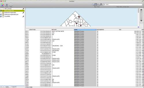
Start by importing the basemap, the public housing data, and the crime incident data by choosing File > Import Vector Data.
To identify the crime locations that are within 200 meters of any public housing location within the city you can use the Spatial Join tool. To accomplish your goals you are going to perform two separate join operations. The first will involve joining crime points to a public housing polygon layer. The second will work backwards to join polygon attributes to crime points. The first join will allow you to create a count of the number of crime points within 200 meters of public housing sites. The second join will allow you to identify what of crimes are near the public housing facilities.
To use the Spatial Join tool you must first select a layer in the Layer Stack that you would like to have data joined to. Begin by selecting the Public Housing layer, and then choose Tools > Spatial Join.
The Spatial Join window has several components that need mentioning. The top of the window details the layers that are available to be joined to the layer selected in the Layer Stack (i.e. Join Layers). Note that the layer you Selected in the Layer Stack is shown in the top Left of the Spatial Join window. The bottom of the window, called the Field Mapping window, contains the fields that are found in both data layers that are going to be joined. In the Field Mapping window pane you can choose to ignore certain fields if you do not want them added to the new vector layer. Additionally, you can select other aggregation options such as copy, min, max, sum, first, last, sum, average, count, and sigma (standard deviation). These options can be applied to any of the field options and they will create a new field in the join layer that has values based on the applied aggregation option. The Ratio checkbox will adjust the attribute data being joined based on the proportionate spatial relationship between the two layers. For example, if a Spatial Join is performed between two neighborhood polygon layers and there is only a 20 percent overlap of the neighborhoods then the joined population variable will be corrected to 20 percent of the original population. The One Feature Per Match option will create an single feature for each spatial match that is made between the layers . The “matching features using” menu allows you to select the type of Spatial Join method that you would like to use. There are many options here that can address your needs in many situations. See below for an example of the Spatial Join Window.
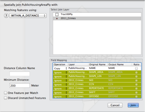
To perform the first join between the Public Housing layer and crime points set up the
Spatial Join window like shown above. First, select the 2011_Crimes layer in the top
windowpane. Within_A_Distance in the Matching Features using menu. Type in 200 in the Minimum
Distance box. In the Field Mapping Pane you want to ignore all of the fields except the Name
field and the Join Count fields (you can highlight all of the items you want to ignore and
type ‘I’ to ignore all). These should be the first and last fields in the Field Mapping
Window. Set those to copy and the rest to ignore and then click Join. A new layer called
PublicHousingAreaPly Join will be added to the layer stack. Click on the layer and observe
the Data Viewer. There should be three fields, ID, Join_Count, and Name.
The Join_Count Field provides the number of crime incidents that occurred within 200 meters of the public housing facilities. The Barry Farm Dwellings had the highest count at 201. Stoddert Terrace is second at 192 and Lincoln Heights Dwelling is third at 182. This information tells you a lot about which public housing facilities might need additional protections against criminal activity, and the data allow you to make compelling statements about what is going on around these facilities.
To perform the second Spatial Join select the2011_Crime layer in the Layer stack and then
choose Tools > Spatial Join. Select the Public Housing Join layer in the top pane of the
Spatial Join window. Change the Matching Features using menu to Within_Distance. Each of the
public housing locations acts as the center of an invisible buffer layer that has a user
defined circumference. To define the circumference of the buffer layer Type in 200 in the
Minimum distance box. Finally, check the Discard Unmatched Features box and then click Join.
This will remove any crime points that are not within 200 meters of a public housing
facility. Move the 2011_Crime join layer to the top of the layer stack. Below is an example
of the map with the selected points.
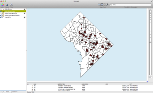
Check the data viewer to find the fields that have been joined to the crime layer. The field of most interest is the Name Field, which describes the name of the public housing site near the crime point. Using this data we can create individual reports for the public housing facilities that details the types of crimes occurring near those facilities. These reports will allows police officials to create goals and strategies for addressing problems in and around these facilities. See below for an example of the data viewer.