With the end of the year approaching everyone is putting out their "Best of" list for 2012. Emily Badger of The Atlantic Cities recently released a list of the "Best Open Data Releases of 2012". These open data sources are available through various agency and government websites and allow users access to data sources that include geospatial data.

We decided to check out a few of the Open Data sources and wanted to create a few maps using Cartographica. The [Philadelphia Open Data website](http:/www.opendataphilly.org/opendata/resource/215/philadelphia-police-part-one- crime-incidents/) was listed as the best Open Data website of 2012. We were able to download a .csv file for all of the crime incidents in Philly since 2006 from the website. Download the Philly Crime data.

To start, add a Live Map to use as a basemap by choosing File > Add Live Map.

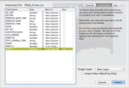
To geocode the data using Cartographica choose File > Import Table Data. The Import File window will appear. Select the coordinates tab in the top right. Change the Map to selection for the Point X and Point Y fields to X (or longitude) and Y (or latitude) and then click Import. See below for an example of the set up.

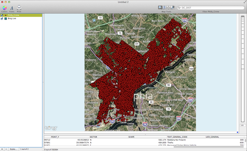
When we geocoded the Philly Crime data 164 incidents were geocoded to the Cincinnati area. Upon further inspection the points were geocoded to the appropriate location based on the data entries. The X and Y coordinates for all of the 164 incorrect points were, -84.69369121 longitude and 39.1207947 latitude, which places the points at the corner of Salyer Ave and Goodrich Lane just West of Cincinnati. These points were considered erroneous and were discarded. To delete the points select them using the identify tool and then choose Edit > Delete.

The map below shows the geocoded crime incident points in Philadelphia since 2006. The Philly_Crime layer contains 592,064 crime points.

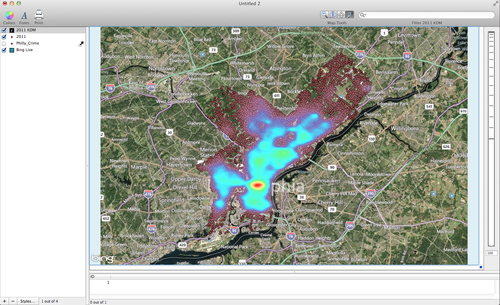
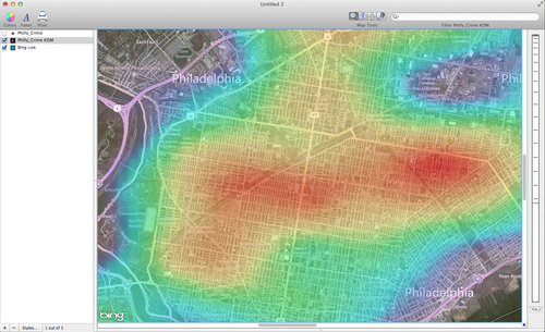
You can filter the data by using the Filter bar. Change the Filter bar selection to Text_General_Code and then type in Homicide. The data will be filtered to only show homicide incident locations. Since 2006, there were 3051 homicides in Philadelphia. Use the identify tool to select all of the points and then hold down the option button and choose Tools > Create Kernel Density Map for Selection. The result of the KDM analysis is shown below. The red areas indicate places where homicide was highly concentrated.

A closer look at central Philadelphia.

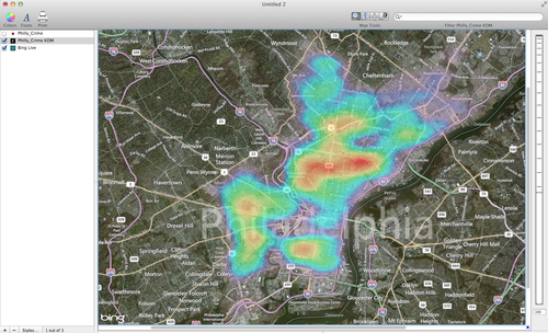
Another way to filter the data is by date. The Philly_Crime layer contains a field called Dispatch_2 that contains the date of the offense. With the Philly Crime layer selected in the layer stack type in 12/31/2010. A small box will appear at the top of the Map Window. You can filter based on multiple criteria to limit the dataset to any year that you want. To select only the 2011 data use the settings shown below. Notice that we are selecting crime incidents that fall between 12/31/2010 and 1/1/2012.

Use the identify tool to select all of the 2011 crime points and then choose Layer > Create Layer from Selection. The new layer should have 82197 crime points. You can repeat these steps so that you can create a new layer for each of the years in the data set. Create another Kernel Density map by Choosing Tools > Create Kernel Density Map. The result of the KDM analysis for the year 2011 data are shown below.