- Mon 07 June 2010
- Cartographica
- Rick Jones
Washington D.C.'s GIS data catalogue provides numerous data about public issues within the city. One interesting data set is crime in D.C. In this post you will see how Cartographica can effectively manage large data sets for use in crime mapping. Specifically, this post will show you how to filter, export, merge, and analyze crime data.
The crime data sets collected from the D.C. GIS catalogue combines many different types of crimes ranging from homicide to theft. Cartographica has the ability to quickly manage and sort data from data sets such as these so that we can easily look at specific crime types. In this example we will look at merging burglary and robbery data so that we can conduct additional analysis on only these two types of crime.
The first part of this example will show you how to filter out and create new layers from the original crime data set. The original data set contains over 37,000 crimes, and our goal here is to create a much smaller data set that only contains the crime types that we want to analyze. Once the data are added the first step is to use the filter bar to select the crime types that we want to merge and then analyze.
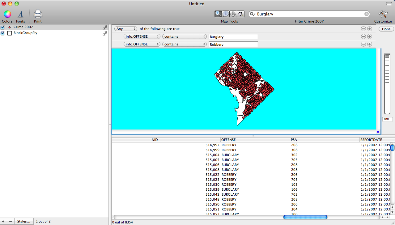
We are interested in Burglary and Robbery so we find the Offense Type field in the filter bar and type in 'Burglary'. You will notice that when you type in burglary into the filter bar a new query bar will appear at the top of the Map Window that gives you options to refine your search. We want the first drop down menu to say 'Any of the following are true', we want the second to say 'info.Offense' (which is the offense field from the crime dataset), we want the third drop down menu to say 'contains' and the last text box we want to type in burglary. Next we want to add a second query to our first by clicking on the plus sign on the right side of the query window on top of the Map Window. A new search box will appear and we want to set the drop down menus to same specifications listed above except we want the text box to have 'Robbery' typed in instead of 'Burglary'. Image one below shows this process. Notice in the tabular data below that the offense field only contains information for Robberies and Burglaries. Also notice that the total number of crimes selected (shown on the bottom of the Cartographica Window where it says 0 out of 8354 indicating that we have selected 0 features out of a total of 8354 total features.
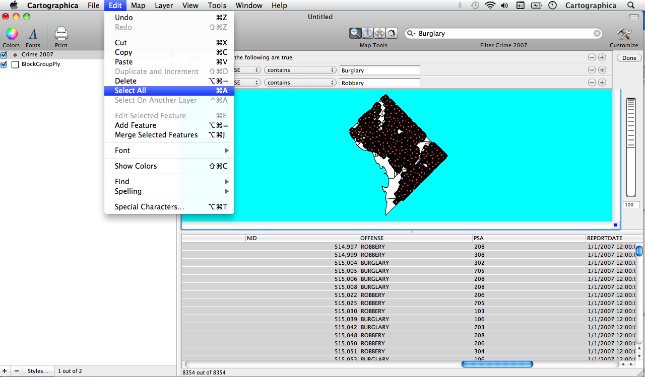
Next we want to select all of the Burglary and Robbery points by clicking on the edit menu and choosing Select All. This will select all of the points on the map. You can verify that the points are selected by looking at the bottom of the Cartographica window and observe that 8354 out of 8354 indicating that all of the points that we queried out are selected. This is shown in Image 2.
Next we want to create a new layer from our selected features. This will complete two steps in one function. We will now create a new layer and merge our Robbery and Burglary information into a new single layer that we can analyze. To do this make sure the points are still selected and then click on the Layer drop down menu and choose Create Layer From Selected Features. Image 3 shows this process.

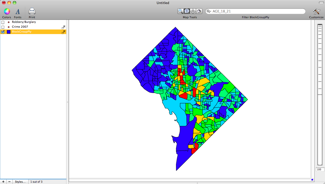
We now have a new layer that is called 'Robbery/Burglary' that we can use for analysis. In order to determine where in D.C. the most robberies and burglaries are committed we can do a couple types of analysis. First we can use Count Points in Polygons and then create a choropleth map to show which block groups in the city have the most trouble with these two types of crime. The Count Points in Polygons tool is found under the Tools drop down menu. Once we have counted the points we can use Cartographica's new Compute Columns feature to construct a rate based on the population within each block group (to see how to Compute Columns click on the link and to see how to build a Choropleth Map click on the link). The image below shows the output from this process
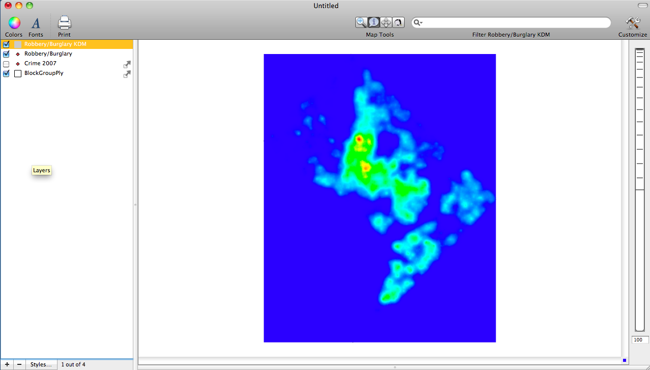
The final type of analysis that can be conducted on our new Robbery/Burglary layer is a Kernel Density Map. Cartographica has a number of Kernels to choose from when conducting this type of analysis each of which has a different effect on the map. To view the different types of kernels click on the Robbery/Burglary layer in the layer stack, click on the tools drop down menu, hold down the option button, and then click on Make Kernel Density Map. This will bring up the Kernel Density Map Window, which will allow you to select your options. The map shown below used the Exponential (Negative) kernel to create the map.