Buffers have many applications for users of GIS. A buffer is a polygon that is drawn at specified distances around a set of point, line, or polygon features. Buffers are often used to indicate the proximity of a feature to other surrounding features. For example, school officials in one community wanted to know which schools were within 500 yards of parks due to increased reports of students skipping school in those locations.

There are different types of buffers, but the most common method is the Uniform Width Buffer. This method identifies areas that are specific distances from a set of features. In the uniform width method the uniform width is applied to all features in a dataset, or to a number of selected features from a dataset.

A useful variant of the Uniform Width Buffer is the Negative Buffer, which is exactly the same as Uniform Width Buffering except that the buffer distances are negative values. Negative buffering is only used with polygons because points and lines have no interior space that can be used to take on negative distance buffers. Polygons on the other hand have interior space that is capable of containing negative distance values. Negative buffers are used to indicate distances toward the center of a polygon from the boundary of the polygon.

Use the following dataset to follow along with this example.

Parcels Dataset

Streets Dataset

Import the data by choosing File > Import Vector Data. For the scenario in this example we have two datasets. One represents a series of polygons for property parcels in a city neighborhood, and the other represents the streets in those neighborhoods. The city needs you to create two polygon layers one representing a 24 foot easement from the centerline of each street and a second polygon representing a 3 foot interior utility easement within each parcel.

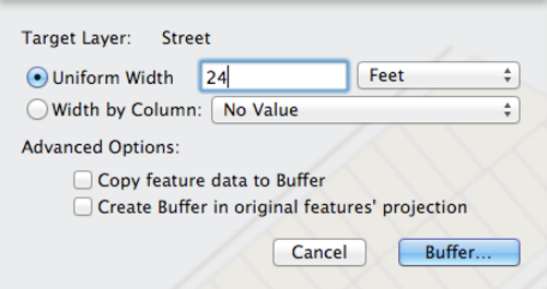
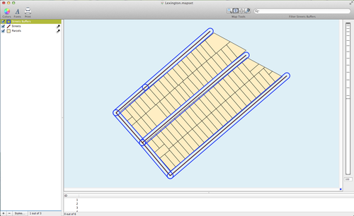
Start with the Street Buffers. Begin by selecting the Streets layer in the Layer Stack. Choose Tools > Create Buffer for Layer's Features. This will bring up the Buffer Window. The Uniform Width option will be selected. Type in 24 and then change the metrics menu to feet. See below for an example of the Buffer Window and the output. You can change the color scheme for the Streets Buffer layer by double-clicking on the layer in the Layer Stack and then changing the fill and stroke color. For the map below the opacity was set to 0%, the stroke color was changed to blue, and the line width was changed to 3.

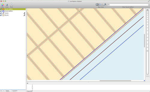
The negative buffer in this scenario represents a 3 foot utility easement that is in place to ensure, among other things, that utility vehicles can get between houses if necessary. The city wants a polygon layer representing these easements. Select the Parcels layer in the Layer Stack and then choose Tools > Create Buffer for Layer's Features. Again, the Buffer Window will appear. This time type in -3, change the metrics menu to feet and then click Buffer... Change the color scheme for the Parcels Buffer Layer by double-clicking on the layer in the Layer Stack. In the map below the fill color was eliminated by changing the opacity to 0%, the stroke color was changed to red, and the line width was changed to 1.5.