- Mon 28 January 2013
- Cartographica
- Rick Jones
- #Contour Maps, #DEM
A new feature in Cartographica version 1.4 is the ability to create contour maps. In GIS, a contour line joins areas of equal elevation above a given level, such as mean sea level. A contour map is a map illustrated with contour lines, which show valleys and hills, and the steepness of slopes. In this sense a contour map can be very useful in many contexts. One method for creating contour lines is by using Digital Elevation Models (DEM). A DEM is a digital model or 3D representation of a terrain's surface — commonly for a planet (including Earth), moon, Mars, or asteroid. Typically DEMs are created based on data that are retrieved through remote sensing technology. Remote sensing technology typically refers to and includes specialized sensors that are attached to various satellites or aerial vehicles that makes observations on the surfaces of their target object.
In this post we emphasize the use of the new contour mapping functions in version 1.4 by using data from the Kentucky Division of Geographic Information. The data on the DGI website are free for download and include DEMs for the entire state of Kentucky. To illustrate the contour mapping we will use data from the Middlesboro, KY area. An interesting geological feature about Middlesboro is that experts believe that its location between Pine Mountain and the Cumberland Mountains is actually an ancient crater from an asteroid impact. This fact makes Middelsboro among the few cities in the world that is seated within an impact crater.
In order to view the entire area for Middlesboro we actually need to download 4 separate DEMs. We need the cells U47, U48, V47, and v48 from the DGI link listed above. To download the DEMs individually control-click within each cell and then select Download Linked File as. Save the Files to your Desktop.
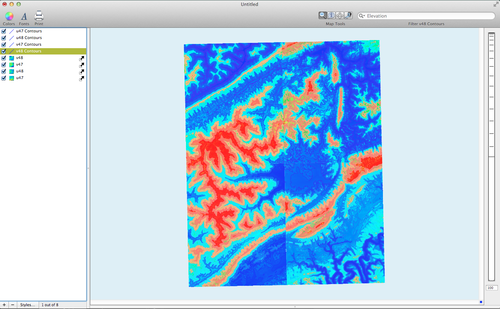
To import the DEMs choose File > Import Raster Data. The following image shows what your map should look like.
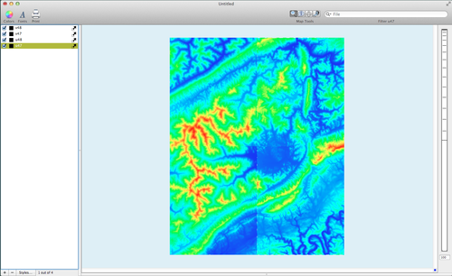
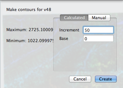
Notice the blue colored circular area near the center of the map. That is the location of Middlesboro and the fairly clear outline of an impact crater. Next, we are going to create contour lines for each of the DEMs that will show the differences in elevations throughout the map. To create contour lines select the DEM layer in the layer stack and then choose Tools > Create Contour Lines. This step has to be done individually for each of the DEM layers. A window will appear that allows you to choose the increments and the base. Select 50 as the increment and leave the base at 0. See below for the contour window.
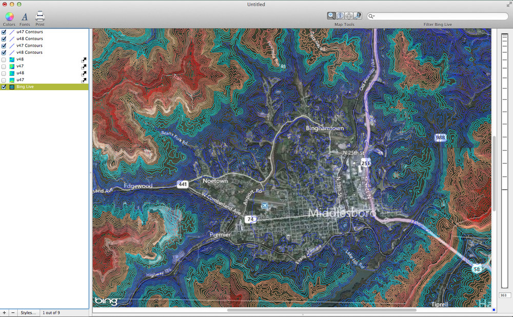
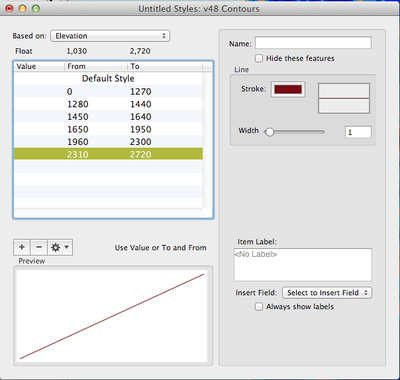
When the contour lines are created they will all be black in color. In order to enhance the visibility of the contours we need to adjust the color schemes. Double-click on the U47 DEM in the Layer Stack. Change the Based on selection to Elevation. Click the + button below the table 6 times and then click the Gear box and select Distribute with Natural Breaks (Jenks). Next, choose Window > Show Uber Browser, click on the Palettes tab, and while holding down the option key click and drag a color palette of your choice into the table within the Layer Styles Window. In the map presented below a blue-red scheme was used where blue = lower elevations and red = higher elevations. Repeat this process for each of the DEMs. See the images below for an example of the Layer Styles window and the map.
Layer Styles Window:
Contour Line Map:
The next image is a closer look at the Impact Basin. Also the following image has the DEM layers turned off and a Live Map added. To add a live map choose File > Add Live Map.