- Wed 19 May 2010
- Tips and Tricks
- Rick Jones
A new feature of Cartographica 1.2 is the ability to re-geocode data that are already added to a map. This new option allows for additional information to be added to a dataset that describes the address used to match the point, a score indicating how accurate the geocoding process was, and a column that describes the source data used for geocoding. These pieces of information are important for keeping track of what went on during geocoding process, which allows for more accurate reporting of analysis results and procedures. Knowing how accurate the geocoding process was along with the specifics about what was matched, gives users the ability to closely monitor their geocoding so that they can ensure that their data is accurate and reliable for use in geospatial analysis.
The new re-geocode feature is important because it allows you to geocode data even when it is not a good match. For example, if an address was mislabeled in past versions of the program it simply would not be geocoded, however now, Cartographica will rematch the mislabeled data, and in doing so will tell you how accurate the match was. This allows you to make judgment call about your data rather than simply not including it at all. Another use of the new re-geocode procedure is that it allows you to verify that data you have collected are accurate. For example, if you collected data from an online data website you can re-geocode the data you collected to be sure that the data meet the accuracy standards that you hope to adhere to during the analysis process. Take a look below to see how to re-geocode data process works.
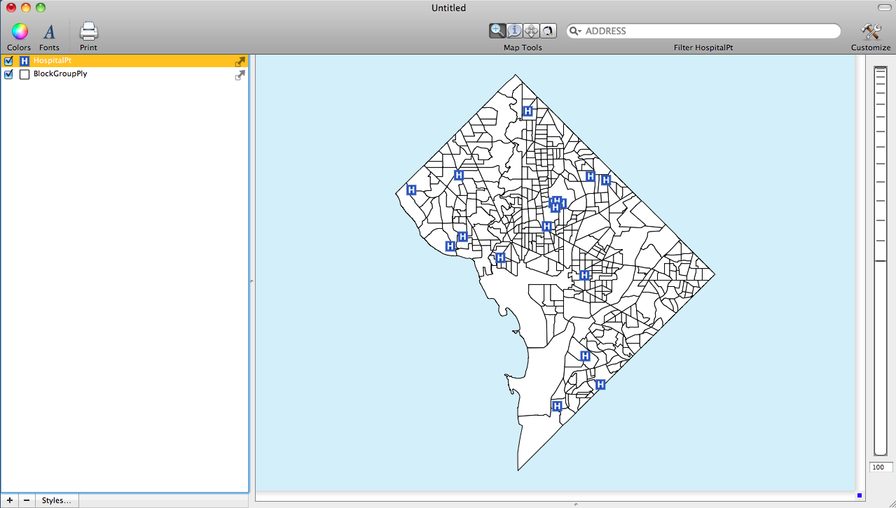
The example below includes data on the Hospitals in Washington D.C. We want to be sure that the points are accurately geocoded.
- The first step is to simply add the data for the Hospitals and the BaseMap
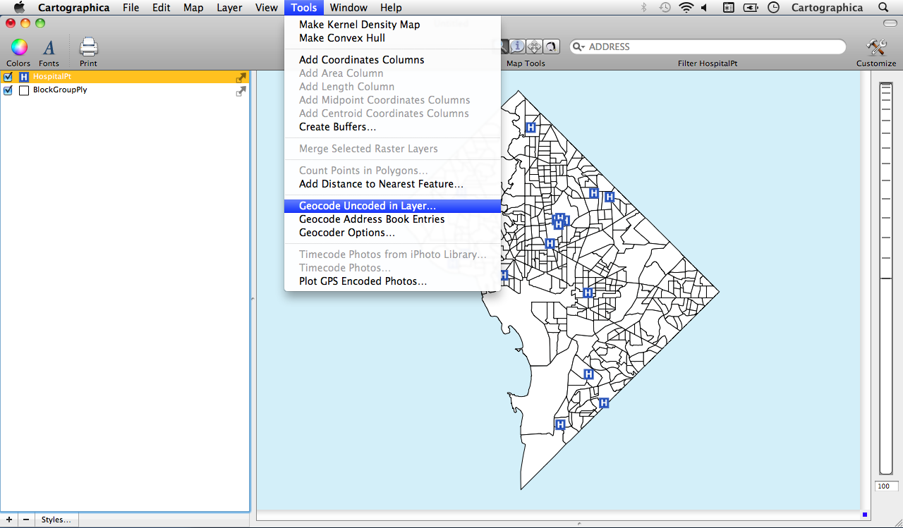
- The second step is to click on Tools, hold down the Option Key and then click on "Geocode Layer...". This will bring up the re-geocode window which allows the user to set the correct address and to choose which information they wish to have added to the Hospital data set. The first screenshot below shows the tools menu before the option key is held down. Once the option key is held down the highlighted portion shown below will change to "Geocode Layer...", which is what we need to re-geocode the data.
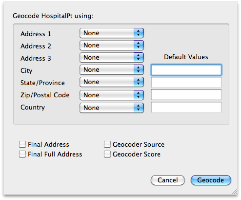
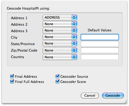
- The third step is to correctly set up the Re-geocode window by choosing the appropriate address column from the Hospitals dataset, then choosing the the information to be added tot he map. The screenshot below shows that we have chosen all four of the new geocoder options.
These options each provide information to the user that explains how the geocoding process was conducted. When the Final Address box is check a new column will be added to the data set that has a "cleaned up" version of the original address imported into the geocoder.
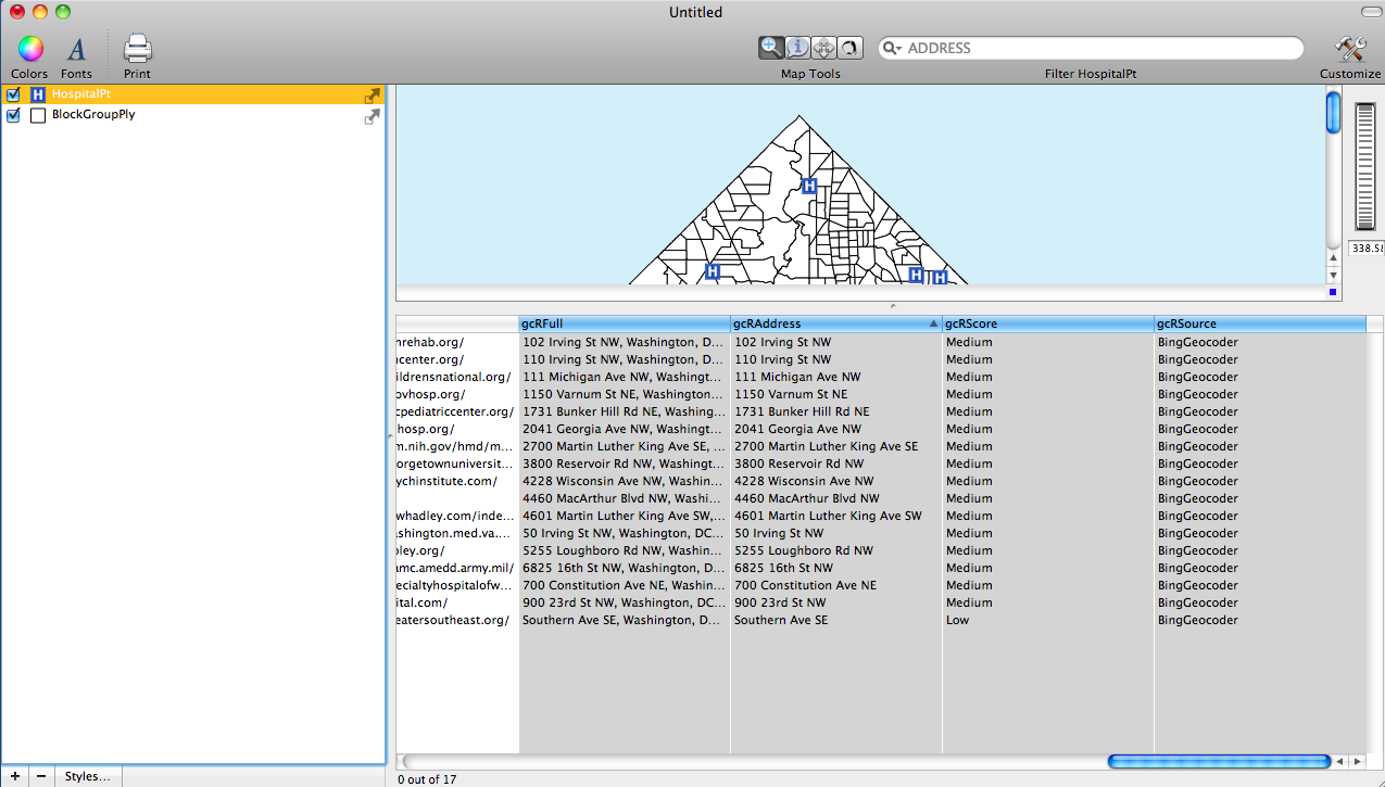
The cleaned up version is based on the street address that was considered to be a match. The Final Full Address includes the full address for the data point rather than just the street address information. The Geocoder Source check box will create a new column in the data set that tell the user the geocoder that was used during the process. This allows the user to know whether the Bing geocoder was used, or if the internal geocoder was used. Finally, the Geocoding Score check box will create a new column that tells the user how accurate the geocoding process was at finding the correct location. Therefore, in the example we want to recode the Metro Stations to see if we can get a high Geocoding score for the points.
A final look at the Hospitals table data shows that there are now four additional columns that contain the information described above